optional: if you want to download the dotnet core SDK in order to build the APIs locally, you can download it from here: https://dotnet.microsoft.com/download
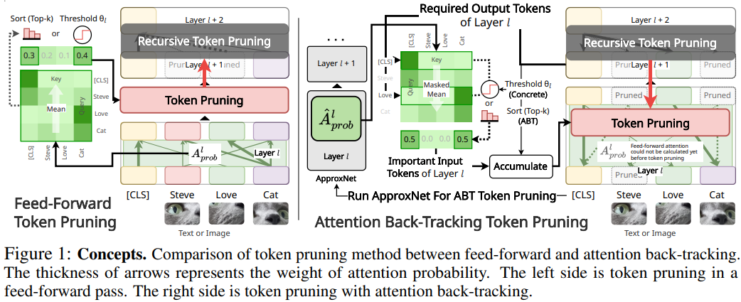
Despite the success of Transformers in various applications from text, vision, and speech domains, they are yet to become standard architectures for mobile and edge device applications due to their heavy memory and computational requirements. While there exist many different approaches to reduce the complexities of the Transformers, such as the pruning of the weights/attentions/tokens, quantization, and distillation, we focus on token pruning, which reduces not only the complexity of the attention operations, but also the linear layers, which have non-negligible computational costs. However, previous token pruning approaches often remove tokens during the feed-forward stage without consideration of their impact on later layers’ attentions, which has a potential risk of dropping out important tokens for the given task. To tackle this issue, we propose an attention back-tracking method that tracks the importance of each attention in a Transformer architecture from the outputs to the inputs, to preserve the tokens that have a large impact on the final predictions. We experimentally validate the effectiveness of the method on both NLP and CV benchmarks, using Transformer architectures for both domains, and the results show that the proposed attention back-tracking allows the model to better retain the full models’ performance even at high sparsity rates, significantly outperforming all baselines. Qualitative analysis of the examples further shows that our method does preserve semantically meaningful tokens.
@inproceedings{
    lee2023sttabt,
    title={Sparse Token Transformer with Attention Back Tracking},
    author={Heejun Lee and Minki Kang and Youngwan Lee and Sung Ju Hwang},
    booktitle={International Conference on Learning Representations},
    year={2023},
    url={https://openreview.net/forum?id=VV0hSE8AxCw}
}
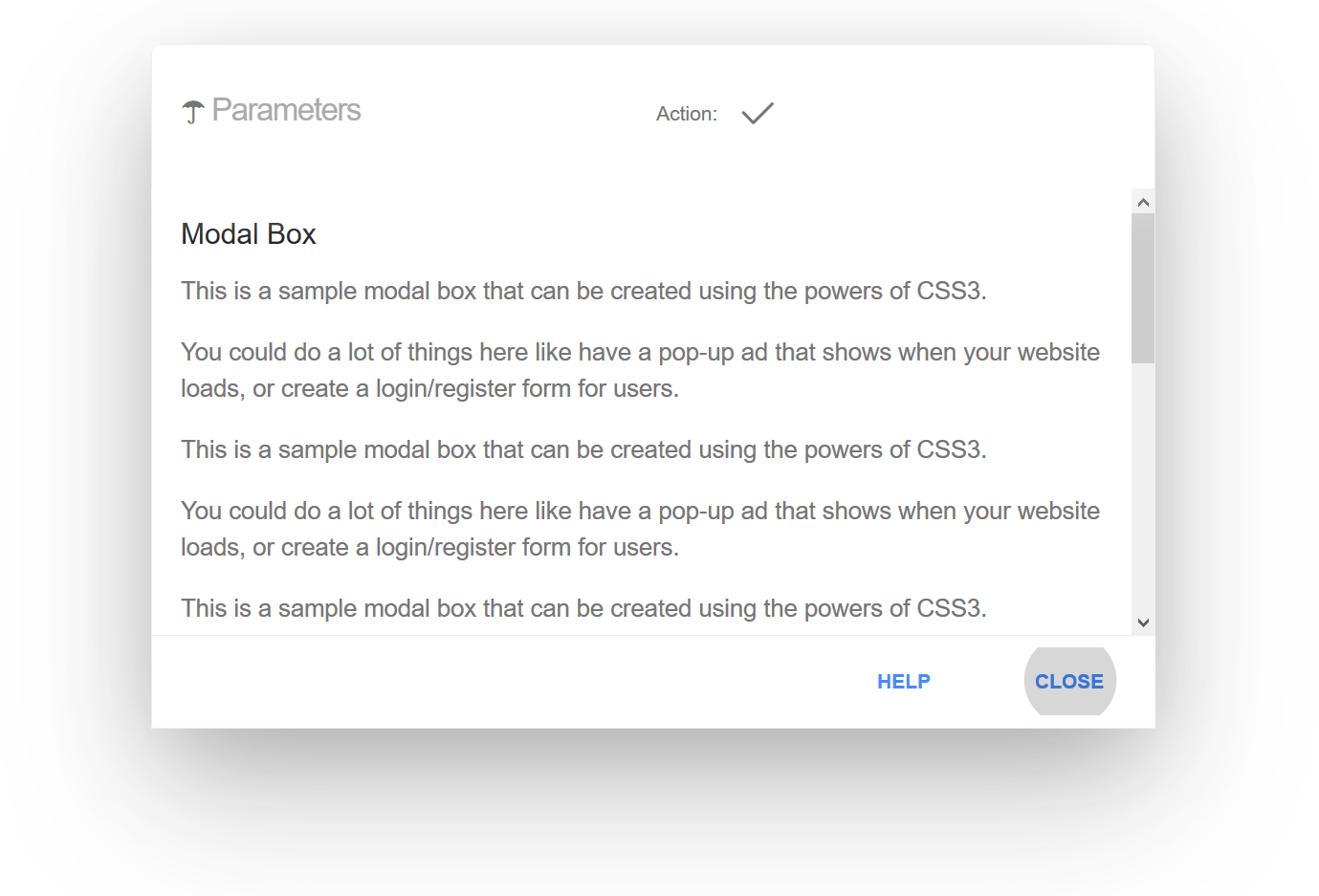
Pure CSS Modal Box, “responsive” with a pretty good browsers support: IE6 minimum! (See this demo here)
Prevents other CSS rules conflicts; animation with Hardware-Accelerated features; fully responsive with width and height support within all screen sizes.
This component template has been tested successfully in (real systems not from emulators):
Internet Explorer 6 (see below);
Internet Explorer 7 (see below);
Internet Explorer 8 (even in regressive ‘Compatibility View’; see below);
Internet Explorer 9;
Internet Explorer 10;
Internet Explorer 11;
Microsoft Edge (all versions);
Internet Explorer (Microsoft Windows Phone 7.5 system);
Safari 5.x;
Safari Mobile;
Opera 9.64 PC;
Opera 11 Linux;
Opera Mini (Microsoft Windows Phone 7.5 system);
Internet Explorer Mobile (Microsoft Windows Phone 8.x system);
Opera Mini for android, version 7.5.x;
Opera Mini android (latest version);
Opera Mini 14 for iOS;
UC Browser (Mini or HD version for Android & normal version for PC);
UC Browser 10.x for iOS;
default browser in Android 2.3.6 (TO DO: font sizes need adaptation);
FireFox 1.0.8 minimum;
FireFox 52 ESR;
Midori 0.4;
Google Chromium (all versions: PC & Mac; iOS & Android);
Brave;
Vivaldi;
Camino 2.1 Mac;
Shiira Mac;
OmniWeb 5 Mac.
Here is a new version with the use of Flexbox & CSS Grid Layout for hipsters and nerds keeping a pretty good support within old browsers: IE6 minimum capable. Please note these new CSS features in this web design sample do not act any kind of noticed advantages. Online latest demo
Usage
First, you need to encapsulate your entire content page into a div with a class name wrapper.
Then, place the Modal Box template outside this wrapper block.
Simple!
Note. The default template is white and blue. For customization, see this sample here
This content package (v1.2 onward)
This minimal default component (required) is distributed in white/blue colors (see screen shots) and do not include the styles for inner optional elements within the modal header (File: modal-box.min.css).
In order to add these additional supports, please include the optional styles (File: custom.css).
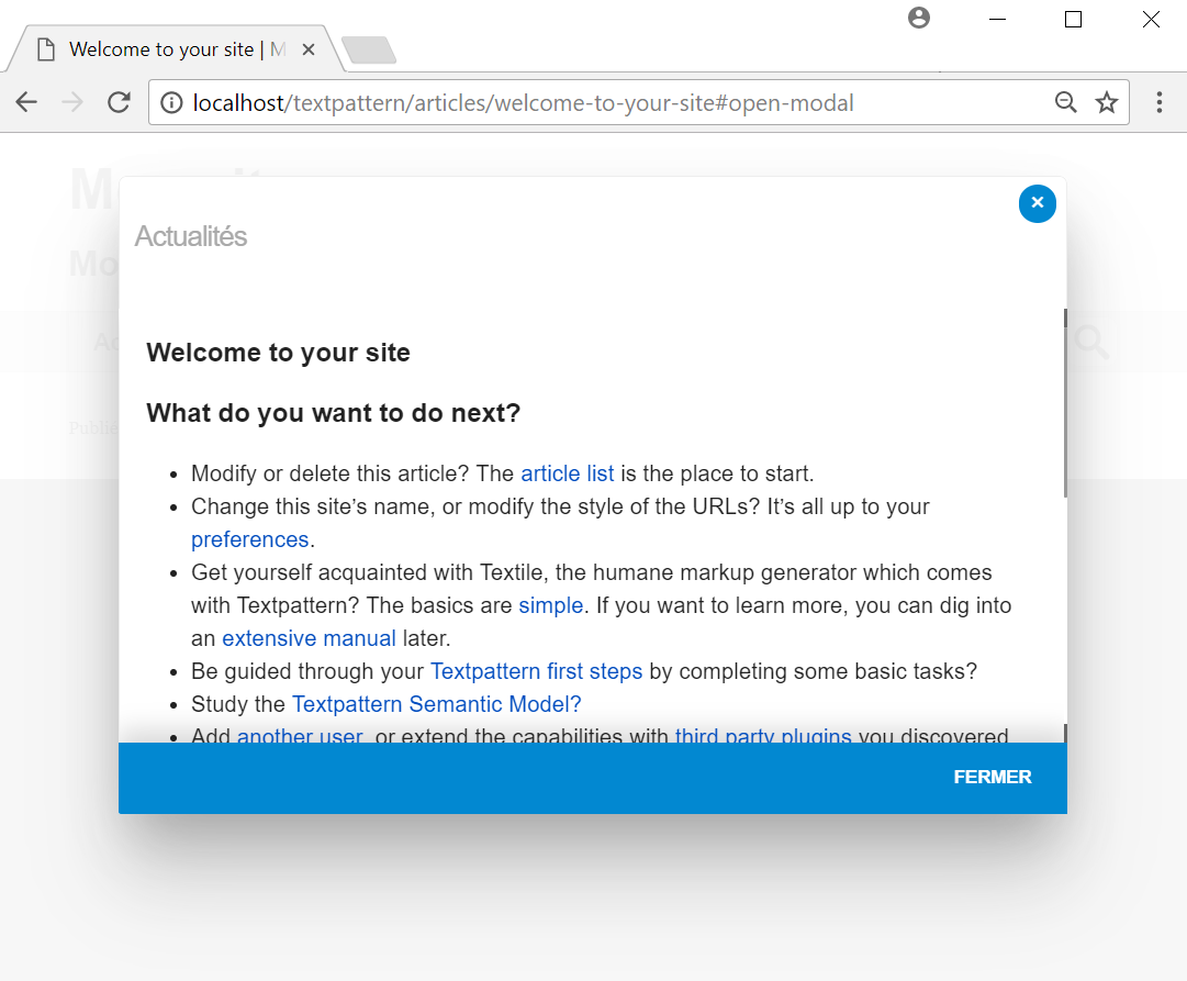
Here is an integration test within the default Textpattern template (v 4.7-dev) without any kind of conflicts even by putting the modal’s styles at the beginning of the default.css file:
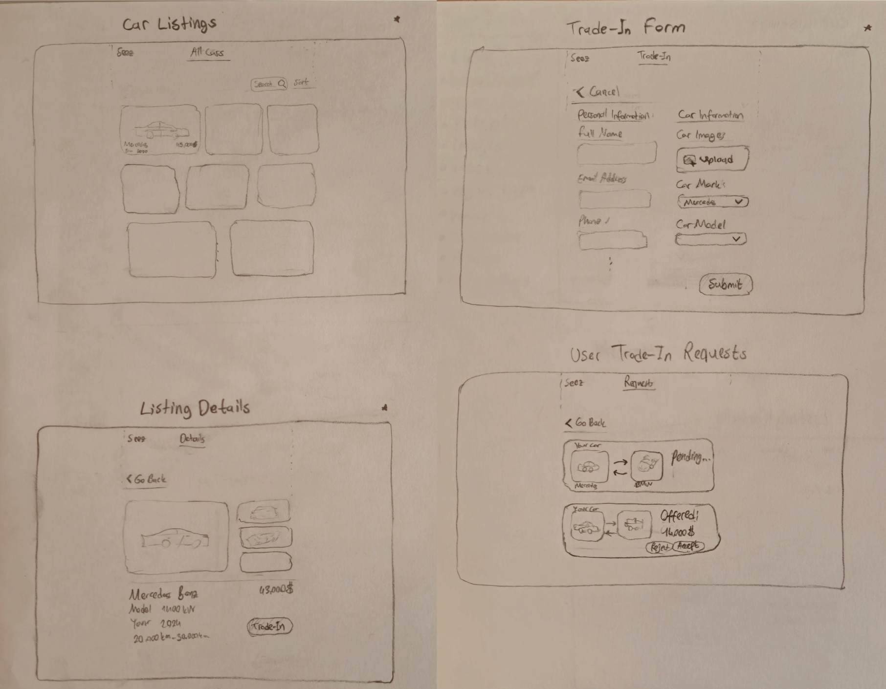
The Car Listings Application is a full-stack web application designed to allow users to browse and interact with car listings. Users can view detailed specifications of cars and apply for trade-ins.
This app uses React, TypeScript, and Tailwind CSS for the frontend, and a Node.js API with PostgreSQL for backend functionality.
You can see the screenshots from the desktop and mobile at the bottom.
init will get mode from process.env or process.argv, read the .env* files, parse the content, handle the inheritance, and reture an object.
dotenv.init()
parse
Parse the content and return an Object with the parsed keys and values.
dotenv.parse(Buffer.from('PROT=3001'))
getConfig
Accept a mode and read .env* files, and handle the inheritance. return finally result.
Example
# Windows Powershell$env:mode="dev"
node .\example\index.mjs
# Mac
mode=dev node ./example/index.mjs
# or
node .\example\index.mjs --mode=dev
Suggest
Add .env.local* in your .gitignore file.
Why not dotenv
When you run your code in multiple environments, you may need some different environments variable. But dotenv didn’t support multiple .env files.
If you don’t use docker or other CI/CD environment variable to instead of .env file, or don’t use shell script to replace .env file, the multiple files is the easiest way to make it work.
For example, your server launched on port 3000, but you want to run on 3001 in local device, the .env file will be shared on repos which used git, so you need a .env.local file, this file has higher-priority then .env and it can doesn’t share with git.
You can create mutiple .env* files, and use them in different environments as easier as possible.
Functional-Input Gaussian Processes with Applications to Inverse
Scattering Problems (Reproducibility)
Chih-Li Sung
December 1, 2022
This instruction aims to reproduce the results in the paper
“Functional-Input Gaussian Processes with Applications to Inverse
Scattering Problems” by Sung et al. (link). Hereafter, functional-Input
Gaussian Process is abbreviated by FIGP.
The following results are reproduced in this file
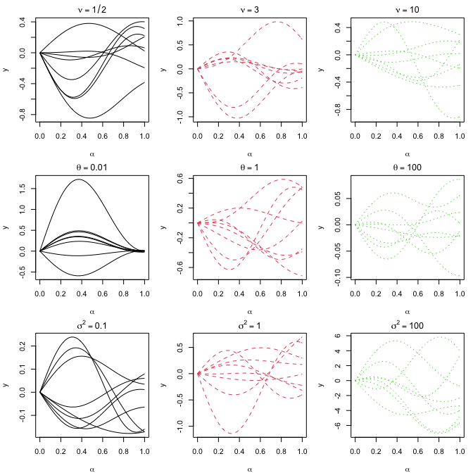
The sample path plots in Section S8 (Figures S1 and S2)
The prediction results in Section 4 (Table 1, Tables S1 and S2)
The plots and prediction results in Section 5 (Figures 2, S3 and S4
and Table 2)
Step 0.1: load functions and packages
library(randtoolbox)
library(R.matlab)
library(cubature)
library(plgp)
source("FIGP.R")                # FIGP
source("matern.kernel.R")       # matern kernel computation
source("FIGP.kernel.R")         # kernels for FIGP
source("loocv.R")               # LOOCV for FIGP
source("KL.expan.R")            # KL expansion for comparison
source("GP.R")                  # conventional GP
Step 0.2: setting
set.seed(1) #set a random seed for reproducingeps<- sqrt(.Machine$double.eps) #small nugget for numeric stability
Reproducing Section S8: Sample Path
Set up the kernel functions introduced in Section 3. kernel.linear is
the linear kernel in Section 3.1, while kernel.nonlinear is the
non-linear kernel in Section 3.2.
with random $\alpha_1,\alpha_2, \beta$ and $\kappa$ from $[0,1]$.
# training functional inputs (G)G<-list(function(x) x[1]+x[2],
function(x) x[1]^2,
function(x) x[2]^2,
function(x) 1+x[1],
function(x) 1+x[2],
function(x) 1+x[1]*x[2],
function(x) sin(x[1]),
function(x) cos(x[1]+x[2]))
n<- length(G)
# y1: integrate g function from 0 to 1y1<- rep(0, n)
for(iin1:n) y1[i] <- hcubature(G[[i]], lower=c(0, 0),upper=c(1,1))$integral# y2: integrate g^3 function from 0 to 1G.cubic<-list(function(x) (x[1]+x[2])^3,
function(x) (x[1]^2)^3,
function(x) (x[2]^2)^3,
function(x) (1+x[1])^3,
function(x) (1+x[2])^3,
function(x) (1+x[1]*x[2])^3,
function(x) (sin(x[1]))^3,
function(x) (cos(x[1]+x[2]))^3)
y2<- rep(0, n)
for(iin1:n) y2[i] <- hcubature(G.cubic[[i]], lower=c(0, 0),upper=c(1,1))$integral# y3: integrate sin(g^2) function from 0 to 1G.sin<-list(function(x) sin((x[1]+x[2])^2),
function(x) sin((x[1]^2)^2),
function(x) sin((x[2]^2)^2),
function(x) sin((1+x[1])^2),
function(x) sin((1+x[2])^2),
function(x) sin((1+x[1]*x[2])^2),
function(x) sin((sin(x[1]))^2),
function(x) sin((cos(x[1]+x[2]))^2))
y3<- rep(0, n)
for(iin1:n) y3[i] <- hcubature(G.sin[[i]], lower=c(0, 0),upper=c(1,1))$integral
Reproducing Table S1
Y<- cbind(y1,y2,y3)
knitr::kable(round(t(Y),2))
y1
1.00
0.33
0.33
1.50
1.50
1.25
0.46
0.50
y2
1.50
0.14
0.14
3.75
3.75
2.15
0.18
0.26
y3
0.62
0.19
0.19
0.49
0.49
0.84
0.26
0.33
Now we are ready to fit a FIGP model. In each for loop, we fit a FIGP
for each of y1, y2 and y3. In each for loop, we also compute LOOCV
errors by loocv function.
loocv.l<-loocv.nl<- rep(0,3)
gp.fit<-gpnl.fit<- vector("list", 3)
set.seed(1)
for(iin1:3){
# fit FIGP with a linear kernelgp.fit[[i]] <- FIGP(G, d=2, Y[,i], nu=2.5, nug=eps, kernel="linear")
loocv.l[i] <- loocv(gp.fit[[i]])
# fit FIGP with a nonlinear kernelgpnl.fit[[i]] <- FIGP(G, d=2, Y[,i], nu=2.5, nug=eps, kernel="nonlinear")
loocv.nl[i] <- loocv(gpnl.fit[[i]])
}
As a comparison, we consider two basis expansion approaches. The first
method is KL expansion.
# for comparison: basis expansion approach# KL expansion that explains 99% of the variance
set.seed(1)
KL.out<- KL.expan(d=2, G, fraction=0.99, rnd=1e3)
B<-KL.out$BKL.fit<- vector("list", 3)
# fit a conventional GP on the scoresfor(iin1:3) KL.fit[[i]] <- sepGP(B, Y[,i], nu=2.5, nug=eps)
The second method is Taylor expansion with degree 3.
# for comparison: basis expansion approach# Taylor expansion coefficients for each functional inputtaylor.coef<-matrix(c(0,1,1,rep(0,7),
rep(0,4),1,rep(0,5),
rep(0,5),1,rep(0,4),
rep(1,2),rep(0,8),
1,0,1,rep(0,7),
1,0,0,1,rep(0,6),
0,1,rep(0,6),-1/6,0,
1,0,0,-1,-1/2,-1/2,rep(0,4)),ncol=10,byrow=TRUE)
TE.fit<- vector("list", 3)
# fit a conventional GP on the coefficientsfor(iin1:3) TE.fit[[i]] <- sepGP(taylor.coef, Y[,i], nu=2.5, nug=eps, scale.fg=FALSE, iso.fg=TRUE)
Let’s make predictions on the test functional inputs. We test n.test
times.
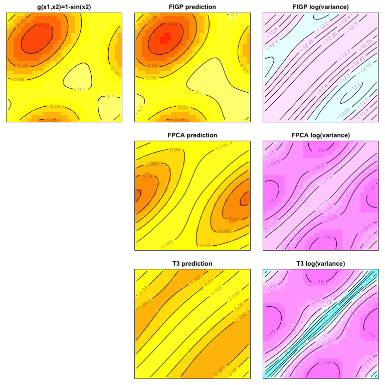
Now we move to a real problem: inverse scattering problem. First, since
the data were generated through Matlab, we use the function readMat in
the package R.matlab to read the data. There were ten training data
points, where the functional inputs are
$g(x_1,x_2)=1$
$g(x_1,x_2)=1+x_1$
$g(x_1,x_2)=1-x_1$
$g(x_1,x_2)=1+x_1x_2$
$g(x_1,x_2)=1-x_1x_2$
$g(x_1,x_2)=1+x_2$
$g(x_1,x_2)=1+x_1^2$
$g(x_1,x_2)=1-x_1^2$
$g(x_1,x_2)=1+x_2^2$
$g(x_1,x_2)=1-x_2^2$
Reproducing Figure 2
The outputs are displayed as follows, which reproduces Figure 2.
We perform PCA (principal component analysis) for dimension reduction,
which shows that only three components can explain more than 99.99%
variation of the data.
ENCM 509 – Fundamentals of Biometric Systems Design Labs
Lab 1
Introduction to libraries such as NumPy, Matplotlib, and SciPy
Lab 2
The purpose of this lab is to utilize statistical analysis to distinguish between “genuine” and “imposter” written signatures. Before applying statistical analysis, we will be collecting written signatures using the Wacom Intuos tablet. We’ll use this tablet to capture coordinate and pressure values at 200 points/sec as the pen moves across the tablet. The tablet is also capable of recognizing 1024 levels of pressure which will be especially useful in statistical analysis later on. In addition, we’ll also utilize the software SigGet to collect and convert the data to CSV files collected by the tablet. Throughout the lab we will utilize these CSV file samples to plot histograms, 2D and 3D colormaps, as well as normal distributions of both velocity and pressure and the calculation of both mean $(\mu)$ and standard deviation $(\sigma)$ in order to understand and compare trends in the distribution/dispersion of the data between both “genuine” and “imposter” written signatures to see how they differ.
Lab 3
The purpose of this lab is to understand biometric-based verification between genuine and imposter signatures for 1:1 matching. In the previous lab, we utilized values such as pressure, time, and coordinates, however, in this lab, we will separate the data into 2 simple classes and train the data based on the EM algorithm. After training the data, we will also utilize the Gaussian Mixture Model (GMM) to calculate log-likelihood scores in order to distinguish the classes of genuine and imposter signatures, essentially “verifying” if the signature is genuine or not. In addition, we will also use the log-likelihood score to calculate both the mean $(\mu)$ and standard deviation $(\sigma)$ of both the imposter and genuine scores in order to plot normal distributions, illustrating how they vary with one another.
Lab 4
In this lab we will be focusing on image pre-processing and feature extraction of fingerprints. We will be collecting fingerprints using the Digital Persona UareU 4500, and because the quality of data is affected by many factors, we will collect both good and bad quality fingerprints for analysis. Throughout the lab we will conduct a number of image processing techniques such as normalization and segmentation as well as pre-processing and de-noising techniques such as contrast enhancement (histogram equalization) and the Wiener filter. After applying these processing techniques, we will then calculate the number of Minutiae (ridge endings and bifurcations) and Singularities (points of cores, deltas) in order to assess their impact on the image details of the fingerprints.
Lab 5
In this lab we will be focusing on image processing and fingerprint matching. We will be using fingerprints collected by using the Digital Persona UareU 4500. We will be focusing on two main matching algorithms, matching based on Minutiae count (ridge ending and bifurcation), and matching based on scores obtained by Gabor filtering. In addition, we will also change the parameters of Gabor filtering such as the angle and frequency in order to see if it has a visual impact on the processed fingerprint image. Lastly, after running both types of matching algorithms, we will also select thresholds in order to see their impact on the number of true positive matches and false negative matches.
Lab 6
In this lab, we will explore facial recognition via Principal Component Analysis (PCA), using the AT&T Database of Faces. Employing Python and Jupyter Notebook, our focus will be on face detection, image processing, and classification through PCA feature extraction and Euclidean Distance matching. We will adjust PCA parameters to study their impact on facial representation and experiment with threshold settings to analyze their effects on true positive and false negative match rates. This practical approach aims to deepen our understanding of biometric verification within facial recognition, blending theoretical concepts with hands-on experience.
Lab 7
In this lab, we will undertake the task of hand gesture recognition using data collected by the Ultra Leap developed by Leap Motion. After the data is collected, we will be utilizing deep learning in order to regonize different hand gestures. More specifically, we will utilize a classifier, Long Short-term Memory (LSTM) which is a deep learning model for time-series analysis. Throughout the lab, we will prepare our data, preprocess it, create our model, and performing classification while also changing specific parameters before classification such as the testing set size, number of LSTM layers, and the dropout probability in order to see their effects on accuracy, etc.
Lab 8
In this lab, we explore Bayesian Networks (BNs) for machine reasoning using PyAgrum.
We’ll construct BNs that mimic real scenarios, like the Diamond Princess infection outbreak.
The lab involves setting up network structures and conditional probability tables (CPTs).
We’ll perform inference to understand how factors like age and gender influence susceptibility.
Exercises in Jupyter Notebook will guide us through these processes.
By manipulating BNs, insights into probabilistic decision-making will be gained.
We aim to show BNs as a robust framework for reasoning under uncertainty.
This practical approach will enhance our comprehension of BNs’ applications.
Ultimately, we’ll learn to make informed decisions based on probabilistic models.
Vonage API – Google Dialogflow integration sample application
This sample application allows you to call a phone number to interact with a Google Dialogflow agent using Vonage Voice API, including getting real time transcripts and sentiment analysis.
This application uses a Dialogflow reference connection code (more details below) for the actual 2-way audio interaction with the Dialogflow agent.
About this sample application
This sample application makes use of Vonage Voice API to answer incoming voice calls and set up a WebSocket connection to stream audio to and from the Dialogflow reference connection for each call.
The Dialogflow reference connection code will:
Send audio to the Dialogflow agent from caller’s speech,
Stream audio responses from the Dialogflow agent to the caller via the WebSocket,
Post back in real time transcripts and caller’s speech sentiment scores via webhooks call back to this Voice API sample application.
Once this application will be running, you call in to the phone number linked to your application (as explained below) to interact via voice with your Dialogflow agent.
Set up the Dialogflow reference connection code – Host server public hostname and port
Default local (not public!) reference connection code port is: 5000.
If you plan to test using Local deployment with ngrok (Internet tunneling service) for both the Dialogflow reference connection code and this sample application, you may set up multiple ngrok tunnels.
For the next steps, you will need:
The Dialogflow reference connection code server’s public hostname and if necessary public port.
e.g. xxxxxxxx.ngrok.io, xxxxxxxx.herokuapp.com, myserver.mycompany.com:32000 (as DF_CONNECTING_SERVER, no port, https:// nor http:// are necessary with ngrok or heroku as public hostname)
Set up your Vonage Voice API application credentials and phone number
Under Capabilities section (click on [Edit] if you do not see this section):
Enable Voice
Under Answer URL, leave HTTP GET, and enter https://<host>:<port>/answer (replace <host> and <port> with the public host name and if necessary public port of the server where this sample application is running)
Under Event URL, select HTTP POST, and enter https://<host>:<port>/event (replace <host> and <port> with the public host name and if necessary public port of the server where this sample application is running)
Note: If you are using ngrok for this sample application, the answer URL and event URL look like: https://yyyyyyyy.ngrok.io/answer https://yyyyyyyy.ngrok.io/event
Click on [Generate public and private key] if you did not yet create or want new ones, save the private.key file in this application folder. IMPORTANT: Do not forget to click on [Save changes] at the bottom of the screen if you have created a new key set.
Link a phone number to this application if none has been linked to the application.
Please take note of your application ID and the linked phone number (as they are needed in the very next section.)
The phone number linked to your application (as SERVICE_NUMBER), your phone will call that number,
The Dialogflow reference connection code server public hostname and port (as DF_CONNECTING_SERVER)
Overview on how this sample Voice API application works
On an incoming call to the phone number linked to your application, GET /answer route plays a TTS greeting to the caller (“action”: “talk”), then start a WebSocket connection to the Dialogflow agent reference connection (“action”: “connect”),
Once the WebSocket is established (GET /ws_event with status “answered”), it plays a TTS greeting to this Dialogflow agent, as the Dialogflow agent expects the user to speak first, we need to start the conversation as one would do in a phone call, with the answerer greeting the caller. The result is that the caller will immediately hear the Dialogflow agent initial greeting (e.g. “How may I help you?”) without having to say anything yet.
You can customize that inital TTS played to Dialogflow to correspond to your Dialogflow agent programming and use case.
Transcripts and sentiment scores will be received by this application in real time,
When the caller hangs up, both phone call leg and WebSocket leg will be automatically terminated.
Running Dialogflow sample Voice API application
You may select one of the following 2 types of deployments.
Local deployment
To run your own instance of this sample application locally, you’ll need an up-to-date version of Node.js (we tested with version 14.3.0).
Download this sample application code to a local folder, then go to that folder.
Copy the .env.example file over to a new file called .env:
cp .env.example .env
Edit .env file, and set the five parameter values:
API_KEY=
API_SECRET=
APP_ID=
SERVICE_NUMBER=
DF_CONNECTING_SERVER=
Install dependencies once:
npm install
Launch the applicatiom:
node df-application
Command Line Heroku deployment
You must first have deployed your application locally, as explained in previous section, and verified it is working.
If you do not yet have a local git repository, create one:
git init
git add .
git commit -am "initial"
Start by creating this application on Heroku from the command line using the Heroku CLI:
heroku create myappname
Note: In above command, replace “myappname” with a unique name on the whole Heroku platform.
On your Heroku dashboard where your application page is shown, click on Settings button,
add the following Config Vars and set them with their respective values:
API_KEY
API_SECRET
APP_ID
SERVICE_NUMBER
DF_CONNECTING_SERVER
add also the parameter PRIVATE_KEY_FILE with the value ./private.key
Now, deploy the application:
git push heroku master
On your Heroku dashboard where your application page is shown, click on Open App button, that hostname is the one to be used under your corresponding Vonage Voice API application Capabilities (click on your application, then [Edit]).
See more details in above section Set up your Vonage Voice API application credentials and phone number.
From any phone, dial the Vonage number (the one in the .env file). This will connect to the DialogFlow agent (as specified in the .env file), and you will be able to have voice interaction with it.
Give CloudWatch Agent permission to publish to CloudWatch
Once the agent is installed, you just need to make sure it has permission to
publish its metrics to CloudWatch. You grant this permission by adding a policy
to the IAM Instance Profile.
Below is an example piece of Terraform code on how to add this to your EC2
profile.
resource"aws_iam_instance_profile""ssm-access-iam-profile" {
name="ec2_profile"role=aws_iam_role.ssm-access-iam-role.name
}
resource"aws_iam_role""ssm-access-iam-role" {
name="ssm-access-role"description="The role to access EC2 with SSM"assume_role_policy=jsonencode({
Version ="2012-10-17"
Statement = [
{
Effect ="Allow"
Principal = {
Service ="ec2.amazonaws.com"
}
Action ="sts:AssumeRole"
}
]
})
}
resource"aws_iam_role_policy_attachment""cloudwatch-policy" {
role=aws_iam_role.ssm-access-iam-role.namepolicy_arn="arn:aws:iam::aws:policy/CloudWatchAgentServerPolicy"
}